Some important (high-level) considerations

In applying any machine learning algorithms to a dataset, several considerations are crucial. This supplementary document covers some of the basic steps in making choices that matter to your problem.

Learning algorithms

Supervised learning

To model relationships and dependencies between input and output.

Regression

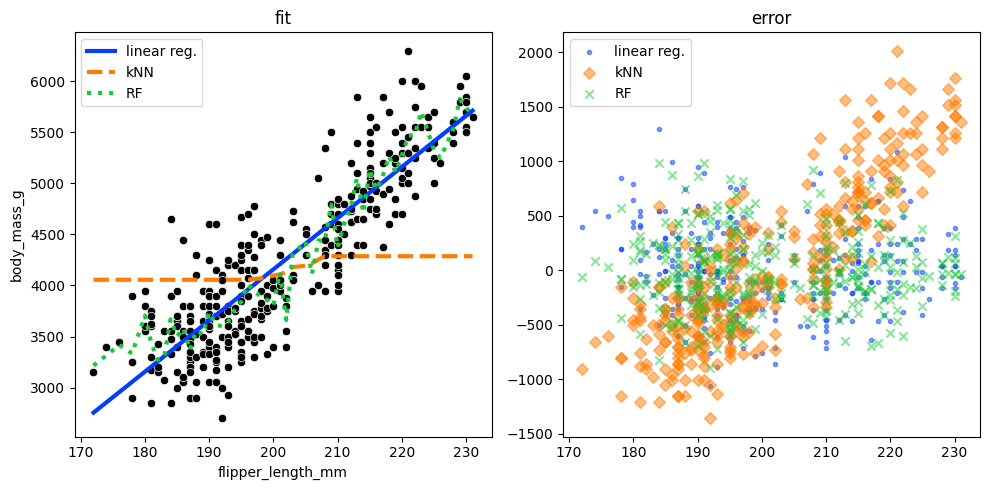
For example, can we predict the mass of a penguin given its other characteristics?

import seaborn as sns
import pandas as pd
sns.set_palette('bright')

penguins = sns.load_dataset('penguins')
penguins = penguins[~penguins.isna().any(axis='columns')]
penguins = penguins.sort_values('flipper_length_mm')

from sklearn.linear_model import LinearRegression
from sklearn.neighbors import KNeighborsRegressor
from sklearn.ensemble import RandomForestRegressor
from sklearn.metrics import root_mean_squared_error

X = penguins[['flipper_length_mm']]
y = penguins['body_mass_g']

# Linear Regression
lr = LinearRegression()
lr.fit(X, y)
y_pred_lr = lr.predict(X)
print(f"Linear Regression RMSE: {root_mean_squared_error(y, y_pred_lr)}")

# Nearest Neighbors
knn = KNeighborsRegressor(n_neighbors=300)
knn.fit(X, y)
y_pred_knn = knn.predict(X)
print(f"Nearest Neighbors RMSE: {root_mean_squared_error(y, y_pred_knn)}")

# Random Forest
rf = RandomForestRegressor()
rf.fit(X, y)
y_pred_rf = rf.predict(X)
print(f"Random Forest RMSE: {root_mean_squared_error(y, y_pred_rf)}")

Linear Regression RMSE: 392.1602706380618
Nearest Neighbors RMSE: 719.5471408610105
Random Forest RMSE: 345.47914963289435

import matplotlib.pyplot as plt
fig, ax = plt.subplots(1, 2, figsize=(10, 5))

sns.scatterplot(y='body_mass_g', x='flipper_length_mm', color='k', data=penguins, ax=ax[0])

y_preds = [y_pred_lr, y_pred_knn, y_pred_rf]
labels = ['linear reg.', 'kNN', 'RF']
linestyles = ['-', '--', ':']
markerstyles = ['.', 'D', 'x']

for j, y_pred in enumerate(y_preds):
    ax[0].plot(X, y_pred, label=labels[j], linestyle=linestyles[j], linewidth=3)
    ax[1].scatter(X, y - y_pred, label=labels[j], marker=markerstyles[j], alpha=0.5)
ax[0].set_title('fit')
ax[1].set_title('error')
ax[0].legend()
ax[1].legend()
plt.tight_layout()

Classification

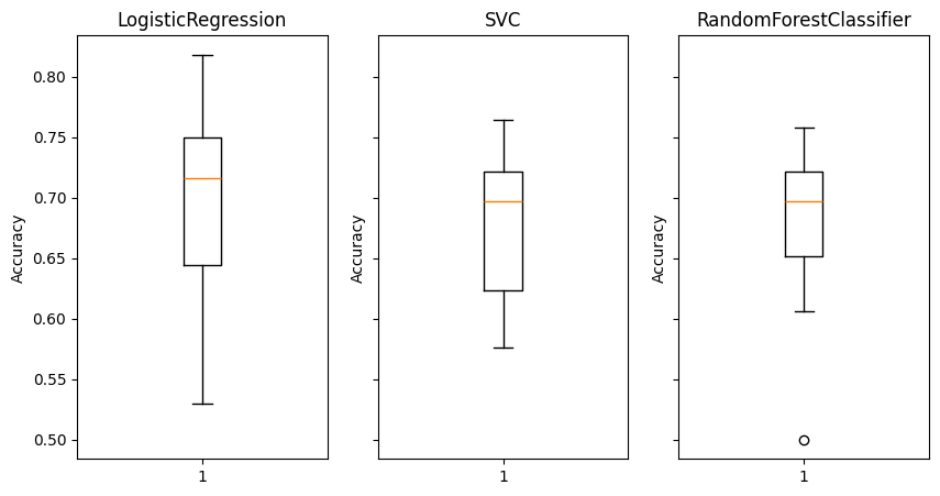
For example, can we predict where a penguin lives given its other characteristics?

def warn(*args, **kwargs):
    pass
import warnings
warnings.warn = warn

from sklearn.linear_model import LogisticRegression
from sklearn.svm import SVC
from sklearn.ensemble import RandomForestClassifier
from sklearn.metrics import accuracy_score
from sklearn.model_selection import cross_val_score
from sklearn.preprocessing import LabelEncoder

# Define inputs and outputs
penguins = penguins.sample(frac=1)
X = penguins.drop("island", axis=1)
y = penguins["island"]

# Encode categorical variables
enc = LabelEncoder()
y = enc.fit_transform(y)
X = pd.get_dummies(X)

models = [LogisticRegression, SVC, RandomForestClassifier]

fig, ax = plt.subplots(1, 3, figsize=(10, 5), sharey=True)
for j, model in enumerate(models):
    m = model()
    cvs = cross_val_score(m, X, y, cv=10)
    ax[j].boxplot(cvs)
    ax[j].set_title(type(m).__name__)
    ax[j].set_ylabel('Accuracy')

Unsupervised learning

To identify structure or relationships.

Clustering

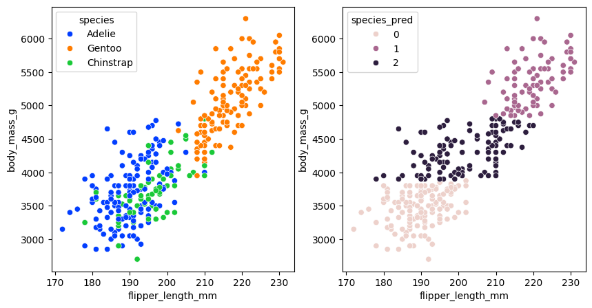
For example, can we group the penguins to identify the species using their characteristics?

from sklearn.cluster import KMeans
from sklearn.metrics import confusion_matrix

# Define input and output
X = penguins.drop(["species", "island", 'sex'], axis=1)
y = penguins["species"]

# Encode categorical variables
enc = LabelEncoder()
y = enc.fit_transform(y)

m = KMeans(n_clusters=3)
m.fit(X)
y_pred = m.predict(X)
penguins['species_pred'] = y_pred

fig, ax = plt.subplots(1, 2, figsize=(10, 5))
sns.scatterplot(y='body_mass_g', x='flipper_length_mm', hue='species', data=penguins, ax=ax[0])
sns.scatterplot(y='body_mass_g', x='flipper_length_mm', hue='species_pred', data=penguins, ax=ax[1])

<Axes: xlabel='flipper_length_mm', ylabel='body_mass_g'>

Semi-supervised learning

Some outputs are “labeled”, most are not, typically in classification problems.

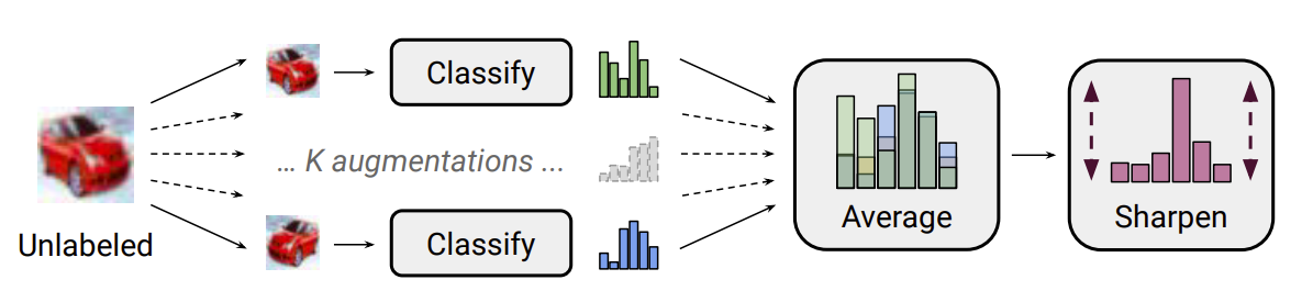
Fig. 10 Example of a semi-supervised learning model [Berthelot et al., 2019].

Reinforcement learning

The algorithm learns by acting and observing reward. The goal is to identify an “optimal” policy.

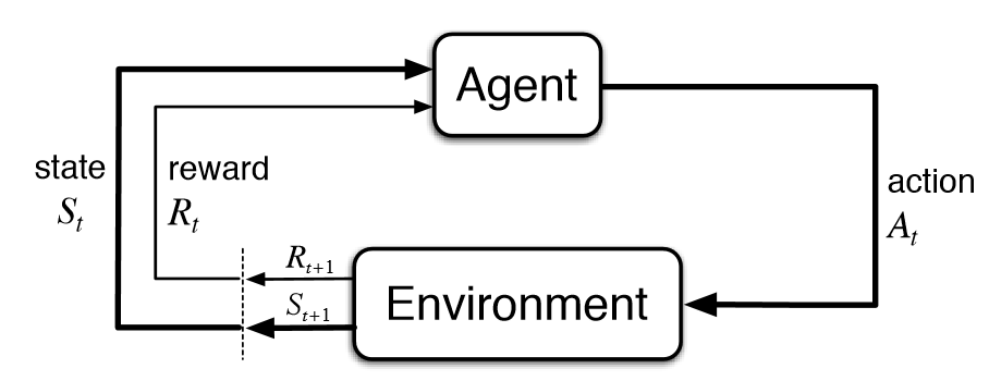
Fig. 11 Generic modeling of a reinforcement learning model.

Practice: diamonds dataset

Consider the diamonds dataset. Specifically, investigate the relationship between price and other variables in the dataset.

Qualitative Answer the modeling process questions:

1. How do we choose a model?

2. How do we quantify the unexplained error?

3. How do we choose the parameters (given data)?

4. How do we evaluate if the model is “good”?

Quantitative

1. Choose two supervised learning models to predict price.

2. Describe the differences between the chosen models.

3. How well does each model perform? Conduct a 10-fold cross validation and report the training and testing performance.

import sklearn
print(sklearn.__version__)

import seaborn as sns

diamonds = sns.load_dataset('diamonds')

1.4.0

Training, testing, and validation

A brief word through https://mlu-explain.github.io/train-test-validation/.

Regularization and hyperparameter tuning

Example: with a linear regression base.

Lasso (\(\ell_1\)):

\[\min_{w} { \frac{1}{2n} ||X w - y||_2 ^ 2 + \alpha ||w||_1}\]

Ridge (\(\ell_2\)):

\[\min_{w} { \frac{1}{2n} ||X w - y||_2 ^ 2 + \alpha ||w||_2 ^ 2}\]

Elastic Net:

\[\min_{w} { \frac{1}{2n} ||X w - y||_2 ^ 2 + \alpha \rho ||w||_1 + \frac{\alpha(1-\rho)}{2} ||w||_2 ^ 2}\]

from sklearn.linear_model import lasso_path, enet_path

X = penguins.drop(['body_mass_g'], axis=1)
X = pd.get_dummies(X)

y = penguins['body_mass_g']

# print("Computing regularization path using the lasso...")
eps = 5e-4
alphas_lasso, coefs_lasso, _ = lasso_path(X, y, eps=eps)
alphas_enet, coefs_enet, _ = enet_path(X, y, eps=eps, l1_ratio=0.8)

import numpy as np 
from itertools import cycle

plt.figure(1)
colors = cycle(["b", "r", "g", "c", "k"])
neg_log_alphas_lasso = -np.log10(alphas_lasso)
neg_log_alphas_enet = -np.log10(alphas_enet)
for coef_l, coef_e, c in zip(coefs_lasso, coefs_enet, colors):
    l1 = plt.plot(neg_log_alphas_lasso, coef_l, c=c)
    l2 = plt.plot(neg_log_alphas_enet, coef_e, linestyle="--", c=c)

plt.xlabel("-Log(alpha)")
plt.ylabel("coefficients")
plt.title("Lasso and Elastic-Net Paths")
plt.legend((l1[-1], l2[-1]), ("Lasso", "Elastic-Net"), loc="lower left")
plt.axis("tight")

Multi-layer ReLU network as an example

Discussion on Section 1.1 in Nonparametric regression on low-dimensional manifolds using deep ReLU networks.