pandas Part II#
This document continues to cover data manipulation with pandas, including aggregation, reorganizing, and merging data.
Grouping data#
Grouping together that are in the same category to aggregate over rows in each category.
Useful in
performing large operations, and
summarizing trends in a dataset.
Say we have a dataset with baby naming frequency throughout the years. Perhaps we are first interested in
how many babies are born in each year? (Good indicator of societal confidence..)
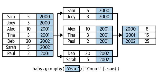
Fig. 1 Example of aggregation in pandas [Lau et al., 2023]#
import pandas as pd

baby = pd.read_csv('../data/ssa-names.csv.zip')
# number of total babies
baby['Count'].sum()
319731698
Grouping and aggregating#
How many babies are born each year?
counts_by_year = baby.groupby('Year')['Count'].sum()
A general recipe for grouping#
(baby                # the dataframe
 .groupby('Year')    # column(s) to group
 ['Count']           # column(s) to aggregate
 .sum()              # how to aggregate
)

# general form
dataframe.groupby(column_name).agg(aggregation_function)
Grouping by multiple attributes#
How many female and male babies are born each year?
counts_by_year_and_sex = baby.groupby(['Year', 'Sex'])['Count'].sum()
counts_by_year_and_sex
Year  Sex
1910  F       352089
      M       164223
1911  F       372382
      M       193441
1912  F       504299
              ...
2019  M      1545678
2020  F      1303090
      M      1478890
2021  F      1320095
      M      1492780
Name: Count, Length: 224, dtype: int64
Aggregating by a custom function#
What about number of unique names by year?
def count_unique(names):
    return len(names.unique())

unique_names_by_year = (baby
 .groupby('Year')
 ['Name']
 .agg(count_unique)           # aggregate using the custom count_unique function
)
unique_names_by_year
Year
1910    1693
1911    1740
1912    2261
1913    2476
1914    2863
        ...
2017    9173
2018    9128
2019    8990
2020    8755
2021    8924
Name: Name, Length: 112, dtype: int64
Apply#
The Series.apply() function applies an arbitrary function on each row entry.
Retrieve first letter of name
def get_first_letter(s):
    return s[0]  # assumes string input
names = baby['Name']
names.apply(get_first_letter)
0          M
1          V
2          E
3          R
4          M
          ..
6311499    Z
6311500    Z
6311501    Z
6311502    Z
6311503    Z
Name: Name, Length: 6311504, dtype: object
Number of letters in name
Quick word about apply() effectiveness#
The apply() function is flexible, accommodating custom operations. But it is slow.
def does_nothing(year):
    return year / 10 * 10
years = baby['Year']
%timeit years / 10 * 10
23.7 ms ± 767 µs per loop (mean ± std. dev. of 7 runs, 10 loops each)
%timeit years.apply(does_nothing)
699 ms ± 8.73 ms per loop (mean ± std. dev. of 7 runs, 1 loop each)
Pivoting#
Pivoting is one way to organize and present data, by arranging the results of a group and aggregation when grouping with two columns.
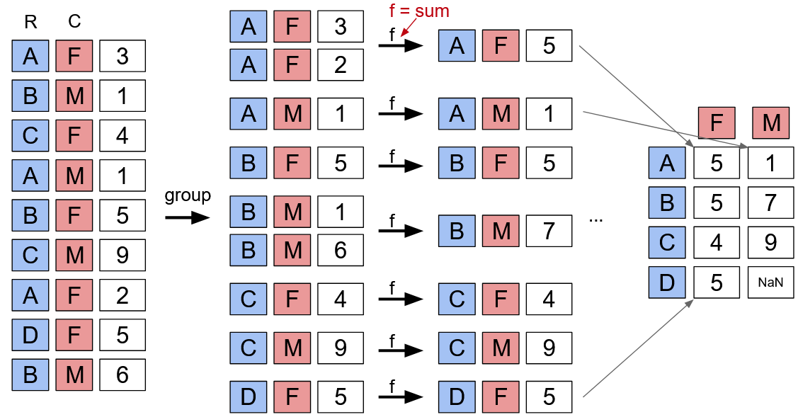
Fig. 2 Example of pivoting in pandas (Data 100)#
mf_pivot = pd.pivot_table(
    baby,
    index='Year',   # Column to turn into new index
    columns='Sex',  # Column to turn into new columns
    values='Count', # Column to aggregate for values
    aggfunc='sum')    # Aggregation function
mf_pivot
| Sex | F | M |
|---|---|---|
| Year | ||
| 1910 | 352089 | 164223 |
| 1911 | 372382 | 193441 |
| 1912 | 504299 | 383704 |
| 1913 | 566973 | 461606 |
| 1914 | 696907 | 596441 |
| ... | ... | ... |
| 2017 | 1405262 | 1606186 |
| 2018 | 1382391 | 1570957 |
| 2019 | 1360299 | 1545678 |
| 2020 | 1303090 | 1478890 |
| 2021 | 1320095 | 1492780 |
112 rows × 2 columns
Melting#
Melting is the “reverse” of pivoting, transforming wide tables into long tables.
mf_long = mf_pivot.reset_index().melt(
    id_vars='Year', # column that uniquely identifies a row (can be multiple)
    var_name='Sex', # name for the new column created by melting
    value_name='Count' # name for new column containing values from melted columns
)
mf_long
| Year | Sex | Count | |
|---|---|---|---|
| 0 | 1910 | F | 352089 |
| 1 | 1911 | F | 372382 |
| 2 | 1912 | F | 504299 |
| 3 | 1913 | F | 566973 |
| 4 | 1914 | F | 696907 |
| ... | ... | ... | ... |
| 219 | 2017 | M | 1606186 |
| 220 | 2018 | M | 1570957 |
| 221 | 2019 | M | 1545678 |
| 222 | 2020 | M | 1478890 |
| 223 | 2021 | M | 1492780 |
224 rows × 3 columns
Why do we need reset_index()?
Practice: Baby Name Data#
Using the baby names data, find the names with most occurrences in each year for both sexes.
baby
| State | Sex | Year | Name | Count | |
|---|---|---|---|---|---|
| 0 | VA | F | 1910 | Mary | 848 |
| 1 | VA | F | 1910 | Virginia | 270 |
| 2 | VA | F | 1910 | Elizabeth | 254 |
| 3 | VA | F | 1910 | Ruth | 218 |
| 4 | VA | F | 1910 | Margaret | 209 |
| ... | ... | ... | ... | ... | ... |
| 6311499 | CA | M | 2021 | Zyan | 5 |
| 6311500 | CA | M | 2021 | Zyion | 5 |
| 6311501 | CA | M | 2021 | Zyire | 5 |
| 6311502 | CA | M | 2021 | Zylo | 5 |
| 6311503 | CA | M | 2021 | Zyrus | 5 |
6311504 rows × 5 columns
Using the meteorite data from the Meteorite_Landings.csv file,
use
groupbyto examine the number of meteors recorded each year.use
groupbyto find the heaviest meteorite from each year and report its name and mass.create a pivot table that shows for each year
the number of meteorites, and
the 95th percentile of meteorite mass.
create a pivot table to compare for each year
the 5%, 25%, 50%, 75%, and 95% percentile of the mass column for the meteorites that were found versus observed falling.
melt the two tables above to create a long-format table.
meteor = pd.read_csv('../data/Meteorite_Landings.csv')
meteor.nametype.unique()
array(['Valid', 'Relict'], dtype=object)
import numpy as np

pivot_table_percentiles = meteor.pivot_table(
    index='year',
    values='mass (g)',
    columns='fall',
    aggfunc=[lambda x: np.percentile(x, 5), lambda x: np.percentile(x, 95)]
)
pivot_table_percentiles
| <lambda> | ||||
|---|---|---|---|---|
| fall | Fell | Found | Fell | Found |
| year | ||||
| 860.0 | 472.000 | NaN | 472.000 | NaN |
| 1399.0 | 107000.000 | NaN | 107000.000 | NaN |
| 1490.0 | 103.300 | NaN | 103.300 | NaN |
| 1491.0 | 127000.000 | NaN | 127000.000 | NaN |
| 1575.0 | NaN | 50000000.00 | NaN | 50000000.00 |
| ... | ... | ... | ... | ... |
| 2010.0 | 100.830 | 1.80 | 4121.000 | 1843.50 |
| 2011.0 | 1445.950 | 3.00 | 13120.000 | 3238.80 |
| 2012.0 | 1087.875 | 25.33 | 2804.625 | 3664.15 |
| 2013.0 | 100000.000 | 37.11 | 100000.000 | 962.20 |
| 2101.0 | NaN | 55.00 | NaN | 55.00 |
245 rows × 4 columns
import numpy as np

pivot_table_95p = meteor.pivot_table(
    index='year',
    values='mass (g)',
    aggfunc=[len, lambda x: np.quantile(x, 0.05), lambda x: np.quantile(x, 0.95)]
)
pivot_table_95p.columns = ['num. of meteorites', '5% percentile of mass', '95% percentile of mass']
pivot_table_95p
| num. of meteorites | 5% percentile of mass | 95% percentile of mass | |
|---|---|---|---|
| year | |||
| 860.0 | 1 | 472.00 | 472.00 |
| 920.0 | 1 | NaN | NaN |
| 1399.0 | 1 | 107000.00 | 107000.00 |
| 1490.0 | 1 | 103.30 | 103.30 |
| 1491.0 | 1 | 127000.00 | 127000.00 |
| ... | ... | ... | ... |
| 2010.0 | 1005 | 1.80 | 2071.60 |
| 2011.0 | 713 | 3.00 | 3381.80 |
| 2012.0 | 234 | 25.39 | 3639.45 |
| 2013.0 | 11 | 37.90 | 50500.00 |
| 2101.0 | 1 | 55.00 | 55.00 |
265 rows × 3 columns
pivot_table_95p.reset_index().melt(
    id_vars='year', # column that uniquely identifies a row (can be multiple)
    var_name='variable', # name for the new column created by melting
    value_name='value' # name for new column containing values from melted columns
)
| year | variable | value | |
|---|---|---|---|
| 0 | 860.0 | num. of meteorites | 1.00 |
| 1 | 920.0 | num. of meteorites | 1.00 |
| 2 | 1399.0 | num. of meteorites | 1.00 |
| 3 | 1490.0 | num. of meteorites | 1.00 |
| 4 | 1491.0 | num. of meteorites | 1.00 |
| ... | ... | ... | ... |
| 790 | 2010.0 | 95% percentile of mass | 2071.60 |
| 791 | 2011.0 | 95% percentile of mass | 3381.80 |
| 792 | 2012.0 | 95% percentile of mass | 3639.45 |
| 793 | 2013.0 | 95% percentile of mass | 50500.00 |
| 794 | 2101.0 | 95% percentile of mass | 55.00 |
795 rows × 3 columns
def p05(x): return np.quantile(x, 0.05)
def p95(x): return np.quantile(x, 0.95)

pivot_table_p = meteor.pivot_table(
    index='year',
    columns='fall',
    values='mass (g)',
    aggfunc=[p05, p95]
)

# Note the use of "stack" due to the multiple levels from the index and columns
pivot_table_p.stack(0, future_stack=True).reset_index()  # future_stack=True is only here for a pandas version issue, it is not necessary
| fall | year | level_1 | Fell | Found |
|---|---|---|---|---|
| 0 | 860.0 | p05 | 472.000 | NaN |
| 1 | 860.0 | p95 | 472.000 | NaN |
| 2 | 1399.0 | p05 | 107000.000 | NaN |
| 3 | 1399.0 | p95 | 107000.000 | NaN |
| 4 | 1490.0 | p05 | 103.300 | NaN |
| ... | ... | ... | ... | ... |
| 485 | 2012.0 | p95 | 2804.625 | 3664.15 |
| 486 | 2013.0 | p05 | 100000.000 | 37.11 |
| 487 | 2013.0 | p95 | 100000.000 | 962.20 |
| 488 | 2101.0 | p05 | NaN | 55.00 |
| 489 | 2101.0 | p95 | NaN | 55.00 |
490 rows × 4 columns