Introduction to (data | statistical | mathematical) modeling

This document covers a general introduction to modeling, for the purpose of inference and prediction.

Zooming out for a second

We have spent significant time in attempting to collect and understand some datasets.

But what about answering the important questions?

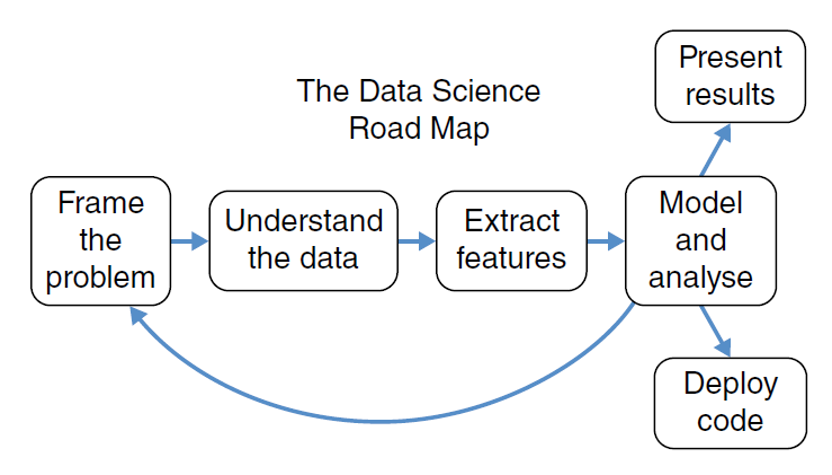
Fig. 4 Data Science Roadmap [Cady, 2017].

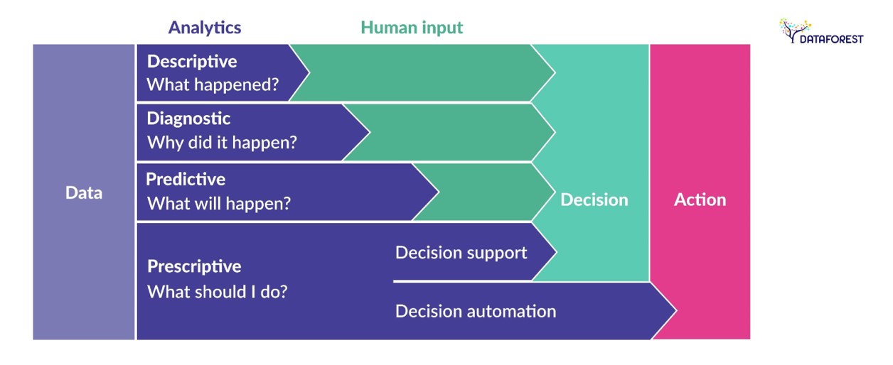
Fig. 5 Types of Data Analytics (DataForest).

What is a model?

A model is a representation of a real (physical) system.

Ball drop example

In one of your physics classes, you may have come across a simple free falling model:

\[ y(t) = - \frac{1}{2} g t^2, \quad v(t) = -g t. \]

import matplotlib.pyplot as plt
import numpy as np
plt.style.use('seaborn-v0_8-colorblind')

# Constants
g = 9.81  # Acceleration due to gravity (m/s^2)
h = 100  # Initial height (m)
t_total = np.sqrt(2*h/g)  # Total time for the ball to hit the ground (s)

# Time array from 0 to t_total
t = np.linspace(0, t_total, num=500)

# Calculate position and velocity as functions of time
y = - 0.5*g*t**2  # Position as a function of time
v = -g*t  # Velocity as a function of time

# Plot position and velocity
plt.figure(figsize=(6, 3))

plt.subplot(1, 2, 1)
plt.plot(t, y, label='Height')
plt.xlabel('Time (s)')
plt.ylabel('Height (m)')
plt.title('Height vs Time')
plt.grid(True)

plt.subplot(1, 2, 2)
plt.plot(t, v, label='Velocity')
plt.xlabel('Time (s)')
plt.ylabel('Velocity (m/s)')
plt.title('Velocity vs Time')
plt.grid(True)

plt.tight_layout()
plt.show()

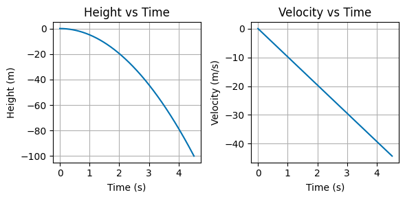
Is this model useful?

Is this model accurate in capturing the freefalling behavior? Why and why not?

What may be a more realistic model?

Why do we build models?

There are three main reasons:

• to explain complex real-world phenomena, (interpretation)

• to predict when there is uncertainty, (accuracy)

• to make causal inference.

Examples (some nuclear physics, some epidemiology)

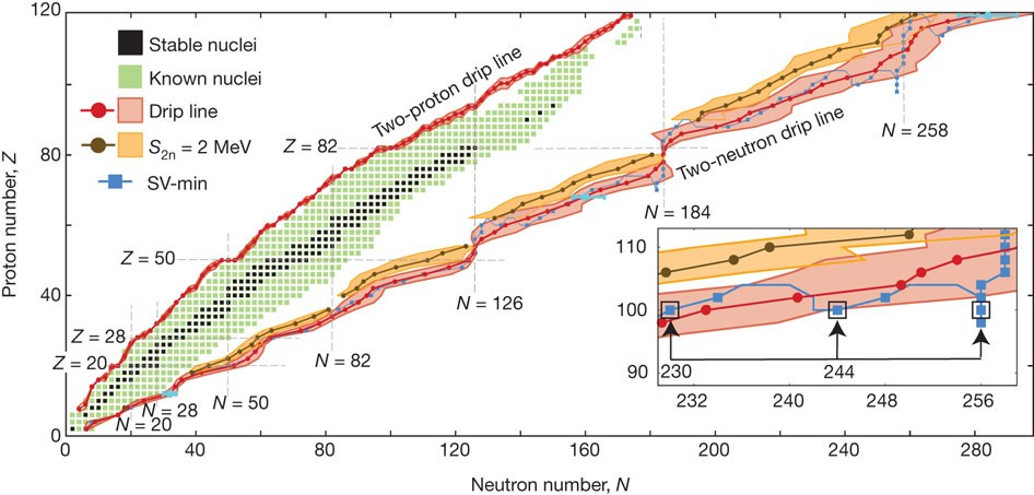
Fig. 6 Even-even nuclei on the nuclear landscape [Erler et al., 2012].

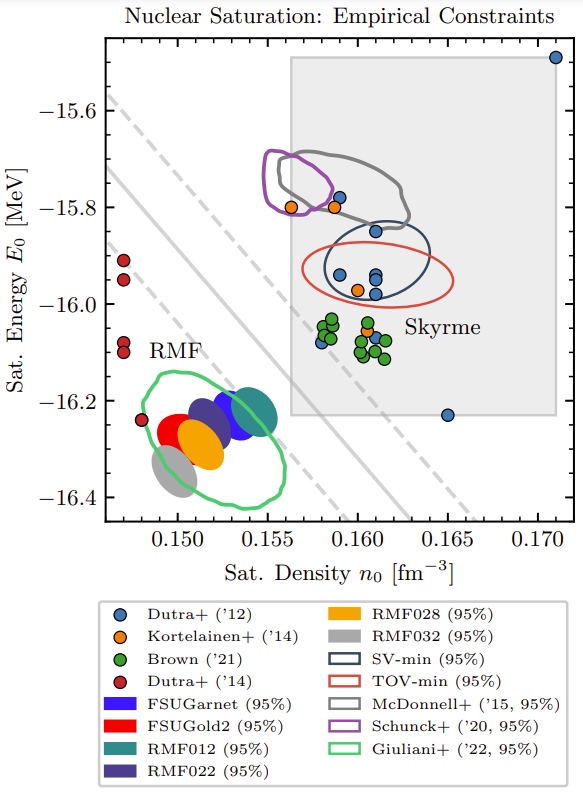
Fig. 7 Summary of empirical constraints of the nuclear saturation point [Drischler et al., 2024].

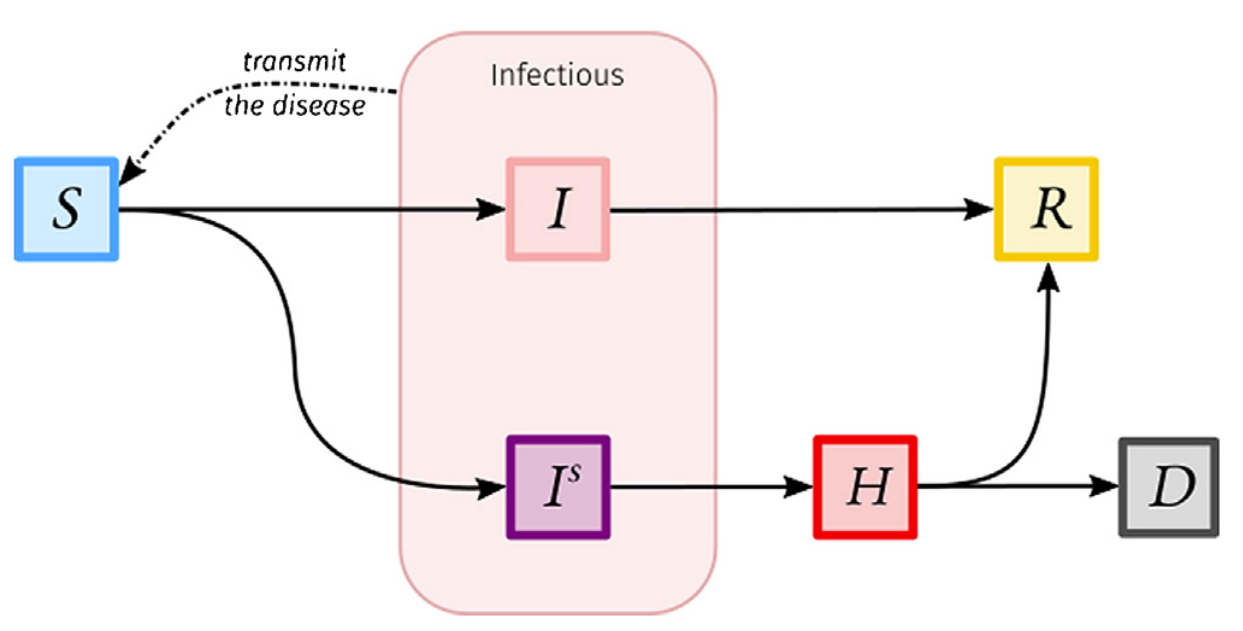
Fig. 8 Example of compartmental model in epidemiology [Reyné et al., 2022].

Modeling process

Consider this very general model:

\[ y = f(x; \theta) + \varepsilon, \text{ where}\]

Notation	Description
\(y\)	output (or outcome, response)
\(x\)	input (or feature, attribute)
\(f\)	model
\(\theta\)	model parameter
\(\varepsilon\)	unexplained error

Questions for any model:

1. How do we choose a model?

2. How do we quantify the unexplained error?

3. How do we choose the parameters (given data)?

4. How do we evaluate if the model is “good”?

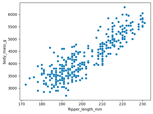
Penguins as an example

Fig. 9 Penguin (www.cabq.gov).

Consider the penguins dataset that has information about 345 penguins.

Perhaps we are interested in the relationship between the length of their flippers and their body mass

#!pip install seaborn
import seaborn as sns
import pandas as pd

penguins = sns.load_dataset('penguins')
# retain complete data
penguins = penguins[~penguins.isna().any(axis='columns')]

sns.scatterplot(y='body_mass_g', x='flipper_length_mm', data=penguins)

<Axes: xlabel='flipper_length_mm', ylabel='body_mass_g'>

Penguins

1. How do we choose a model?

Say we select the following linear model:

\[ y_i = \beta_0 + \beta_1 x_i + \varepsilon_i.\]

2. How do we quantify the unexplained error?

The errors, as a result of the model choice, is

\[ \varepsilon_i = y_i - (\beta_0 + \beta_1 x_i).\]

3. How do we choose the parameters (given data)?

A common way to select the parameters is to minimize errors, specified by a loss function. Loss functions are designed to evaluate how good a parameter is.

For examples, both of the following would be a legitimate loss function, with respect to \(\boldsymbol{\beta}\):

\[ \ell_1(\boldsymbol{\beta}) = \sum_{i=1}^n |y_i - (\beta_0 + \beta_1 x_i)|, \]

\[ \ell_2(\boldsymbol{\beta}) = \sum_{i=1}^n (y_i - (\beta_0 + \beta_1 x_i))^2. \]

y = penguins.body_mass_g.values
x = penguins.flipper_length_mm.values

def l1_loss(beta, x, y):
    return np.sum(np.abs(y - beta[0] - beta[1]*x))

import numpy as np

beta = np.array((0, 1))  # a "guess"

l1_loss(beta, x, y)

1334028.0

# FILL-IN: write the l2_loss function and return the l2_loss where beta = np.array((0, 1))
def l2_loss():
    return

Under the hood of “fitting”:

Given a loss function, the fitting step means to find a set of parameters that minimizes the loss. Inheritly, it is an optimization.

import scipy

beta0 = beta
l1_opt = scipy.optimize.minimize(l1_loss, beta0, args=(x, y))

l1_opt

  message: Desired error not necessarily achieved due to precision loss.
  success: False
   status: 2
      fun: 103608.94055436643
        x: [-5.984e+03  5.060e+01]
      nit: 15
      jac: [-1.000e+00 -2.080e+02]
 hess_inv: [[ 1.082e+01 -5.738e-02]
            [-5.738e-02  3.065e-04]]
     nfev: 210
     njev: 69

# FILL-IN: find the optimal parameters using the l2_loss function.
def l2_loss(beta, x, y):
    return np.sum((y - beta[0] - beta[1]*x)**2)
l2_opt = scipy.optimize.minimize(l2_loss, beta0, args=(x, y))

l2_opt

  message: Optimization terminated successfully.
  success: True
   status: 0
      fun: 51211962.729684055
        x: [-5.872e+03  5.015e+01]
      nit: 6
      jac: [ 0.000e+00  0.000e+00]
 hess_inv: [[ 3.113e-01 -1.542e-03]
            [-1.542e-03  7.671e-06]]
     nfev: 33
     njev: 11

# An alternative way to find the optimal parameters with l2_loss.
x_mat = np.array((np.ones(x.shape[0]), x)).T
beta_l2_opt = np.linalg.solve(x_mat.T @ x_mat, x_mat.T @ y)

beta_l2_opt

array([-5872.09268284,    50.15326594])

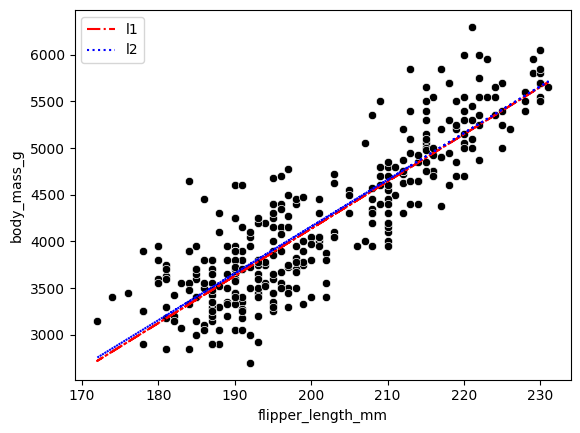
4. How do we evaluate if the model is “good”?

import matplotlib.pyplot as plt

fig, ax = plt.subplots(1, 1)
sns.scatterplot(y='body_mass_g', x='flipper_length_mm', color='k', data=penguins, ax=ax)
ax.plot(x, l1_opt.x[0] + l1_opt.x[1] * x, color='red', linestyle='-.', label='l1')
ax.plot(x, l2_opt.x[0] + l2_opt.x[1] * x, color='blue', linestyle=':', label='l2')
plt.legend()

<matplotlib.legend.Legend at 0x3e90cbd0>

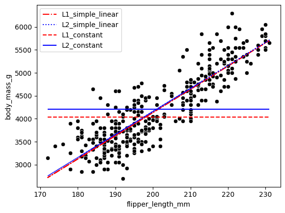
(Why not) try a constant model?

\[y_i = \beta_0 + \varepsilon_i.\]

def l1_constant_loss(beta, y):
    return np.sum(np.abs(y - beta))
def l2_constant_loss(beta, y):
    return np.sum((y - beta)**2)
    
l1_constant_opt = scipy.optimize.minimize(l1_constant_loss, 0, args=y)
l2_constant_opt = scipy.optimize.minimize(l2_constant_loss, 0, args=y)

fig, ax = plt.subplots(1, 1)
sns.scatterplot(y='body_mass_g', x='flipper_length_mm', color='k', data=penguins, ax=ax)
ax.plot(x, l1_opt.x[0] + l1_opt.x[1] * x, color='red', linestyle='-.', label='L1_simple_linear')
ax.plot(x, l2_opt.x[0] + l2_opt.x[1] * x, color='blue', linestyle=':', label='L2_simple_linear')
ax.hlines(y=l1_constant_opt.x, xmin=np.min(x), xmax=np.max(x), color='red', linestyle='--', label='L1_constant')
ax.hlines(y=l2_constant_opt.x, xmin=np.min(x), xmax=np.max(x), color='blue', linestyle='-', label='L2_constant')
plt.legend()

<matplotlib.legend.Legend at 0x3e725790>

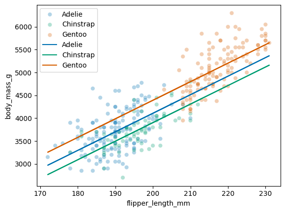
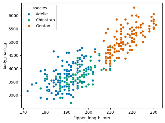
What if we are shown this graph though?

sns.scatterplot(y='body_mass_g', x='flipper_length_mm', hue='species', data=penguins)

<Axes: xlabel='flipper_length_mm', ylabel='body_mass_g'>

# categorial predictor?
from sklearn.preprocessing import OneHotEncoder

enc = OneHotEncoder()
species_onehot = enc.fit_transform(penguins[['species']]).todense()

\[y_i = \beta_0 + \beta_1 \text{[flipper\_length\_mm]} + \beta_2 \text{[is\_adelie]} + \beta_3 \text{[is\_chinstrap]} + \beta_4 \text{[is\_gentoo]}\]

# Form the design matrix
X = np.array((np.ones(x.shape[0]), x)).T

X = np.column_stack((X, species_onehot))

X = np.array(X)
X

array([[  1., 181.,   1.,   0.,   0.],
       [  1., 186.,   1.,   0.,   0.],
       [  1., 195.,   1.,   0.,   0.],
       ...,
       [  1., 222.,   0.,   0.,   1.],
       [  1., 212.,   0.,   0.,   1.],
       [  1., 213.,   0.,   0.,   1.]])

from sklearn.linear_model import LinearRegression

reg = LinearRegression(fit_intercept=False)

reg.fit(X, y)

betas = reg.coef_
betas

array([-2990.09713522,    40.60616529, -1023.08175274, -1228.45723258,
        -738.5581499 ])

fig, ax = plt.subplots(1, 1)
sns.scatterplot(y='body_mass_g', x='flipper_length_mm', hue='species', data=penguins, alpha=0.3)
for i in range(2, 5):
    ax.plot(x, betas[0] + betas[1]*x + betas[i], label=enc.categories_[0][i-2])
plt.legend()

<matplotlib.legend.Legend at 0x3eb36450>