Intro to EDA

Published

April 7, 2026

Exploratory data analysis, or EDA, is a standard practice prior to any data manipulation and analysis.

Recall that data engineering is primarily about data preparation to serve smooth and effective data analysis. Exploratory data analysis generally refers to the step of understanding the data:

summarizing characteristics of raw data
visualizing data (single and multiple variables)
identifying missing data
identifying outliers

This document primarily deals with the first two items.

Goals

In the exploratory phase, these are for people behind the scenes to see.

The main goals here are:

capture main message
(relatively) quick exploration across many summaries (including plots)
not intended for a client or presentation

What does this translate to, technically?

each summary should have meaningful information
label your plots

Data summary

As a starting point, simply looking at the data is worth the while. Some common questions to consider are the following:

General dataset info: size, dtypes
Missing values?
Duplicate data?
Continuous variables
Categorical variables
Bivariate relationships
Potential data quality issues, e.g., inconsistency, special NA characters

# !pip install pandas seaborn matplotlib

import pandas as pd
import seaborn as sns
import matplotlib.pyplot as plt


The origin of sns.

Earthquake dataset

Source Link

# load and save a copy of the earthquake dataset
earthquake = pd.read_csv('https://raw.githubusercontent.com/mosesyhc/de300-2026wi/refs/heads/main/datasets/Canadian-Earthquakes-2010-2019.csv')

# take a glimpse of the data
earthquake.head()

	magnitude_codelist	magnitude	magnitude_type	date	place	depth	latitude	longitude	OBJECTID	longitude_geom	latitude_geom
0	<2	1.7	ML	2010-01-01T00:16:49+0000	81 km NE of Seattle	0.0	48.192001	-121.677002	1	-121.677315	48.191706
1	2	2.2	MN	2010-01-01T00:52:50+0000	86 km NW from Maniwaki	18.0	47.028999	-76.583000	2	-76.583303	47.028909
2	<2	1.8	MN	2010-01-01T03:21:58+0000	21 km NW from Mont-Laurier	18.0	46.651001	-75.734001	3	-75.733902	46.650809
3	<2	1.5	MN	2010-01-01T04:14:51+0000	CHARLEVOIX SEISMIC ZONE	13.0	47.740002	-69.741997	4	-69.742000	47.740210
4	<2	1.6	ML	2010-01-01T04:15:17+0000	83 km W of Gold R.	11.6	49.500999	-127.222000	5	-127.222216	49.500705

# view a summary of the full data
earthquake.info()

<class 'pandas.DataFrame'>
RangeIndex: 44561 entries, 0 to 44560
Data columns (total 11 columns):
 #   Column              Non-Null Count  Dtype  
---  ------              --------------  -----  
 0   magnitude_codelist  44561 non-null  str    
 1   magnitude           44561 non-null  float64
 2   magnitude_type      44462 non-null  str    
 3   date                44561 non-null  str    
 4   place               44561 non-null  str    
 5   depth               44561 non-null  float64
 6   latitude            44561 non-null  float64
 7   longitude           44561 non-null  float64
 8   OBJECTID            44561 non-null  int64  
 9   longitude_geom      44561 non-null  float64
 10  latitude_geom       44561 non-null  float64
dtypes: float64(6), int64(1), str(4)
memory usage: 5.8 MB

# checks for duplicates (also ask if duplicates make sense)
earthquake.duplicated()

# .loc / .iloc

0        False
1        False
2        False
3        False
4        False
         ...  
44556    False
44557    False
44558    False
44559    False
44560    False
Length: 44561, dtype: bool

# duplicates

# a quick numerical summary 
earthquake.describe(include='all')

	magnitude_codelist	magnitude	magnitude_type	date	place	depth	latitude	longitude	OBJECTID	longitude_geom	latitude_geom
count	44561	44561.000000	44462	44561	44561	44561.000000	44561.000000	44561.000000	44561.000000	44561.000000	44561.000000
unique	6	NaN	7	44481	18639	NaN	NaN	NaN	NaN	NaN	NaN
top	<2	NaN	ML	2018-07-02T04:08:13+0000	CHARLEVOIX SEISMIC ZONE	NaN	NaN	NaN	NaN	NaN	NaN
freq	19764	NaN	29509	3	1250	NaN	NaN	NaN	NaN	NaN	NaN
mean	NaN	2.134070	NaN	NaN	NaN	12.852194	53.351863	-118.953322	22281.000000	-118.953299	53.351830
std	NaN	0.828096	NaN	NaN	NaN	9.963145	6.214464	23.696484	12863.797009	23.696493	6.214465
min	NaN	-1.400000	NaN	NaN	NaN	-0.500000	40.808998	-148.811005	1.000000	-148.810526	40.808509
25%	NaN	1.600000	NaN	NaN	NaN	5.000000	49.169998	-132.427994	11141.000000	-132.427618	49.170009
50%	NaN	2.100000	NaN	NaN	NaN	10.000000	52.137001	-129.671997	22281.000000	-129.672016	52.136507
75%	NaN	2.700000	NaN	NaN	NaN	18.000000	56.514999	-121.947998	33421.000000	-121.948318	56.515206
max	NaN	7.700000	NaN	NaN	NaN	214.000000	82.608002	-39.320000	44561.000000	-39.319968	82.607812

# checks for possible statistical assumption(s)
import scipy.stats as sps

sps.normaltest(earthquake['magnitude'])

NormaltestResult(statistic=np.float64(1597.6658124732553), pvalue=np.float64(0.0))

# extract only numeric variables
earthquake

# for example, normality test
sps.shapiro(earthquake['magnitude'])

C:\Users\moses\AppData\Local\Programs\Python\Python312\Lib\site-packages\scipy\stats\_axis_nan_policy.py:592: UserWarning: scipy.stats.shapiro: For N > 5000, computed p-value may not be accurate. Current N is 44561.
  res = hypotest_fun_out(*samples, **kwds)

ShapiroResult(statistic=np.float64(0.9877396508026011), pvalue=np.float64(1.179774985585813e-49))

# for example, another normality test

# pairwise correlation
earthquake_num = earthquake.select_dtypes('number')
import numpy as np
np.corrcoef(earthquake_num.iloc[:500])

Data visualization

sns.set(context='talk', style='ticks')  # simply for aesthetics
sns.set_palette('magma')
%matplotlib inline 

# earthquake = earthquake.sample(n=500)  # (if too slow) for illustration purposes

# histogram for continuous variables using pandas built-in plots

# relative frequency? ...

# histogram of masses by group

# other types of plots

# counts for categorical variables

# barplots by group

# bivariate plots

# bivariate plots (log-log)

# pairwise plots  (time-consuming)

# another pairwise plot by group

In-class activity

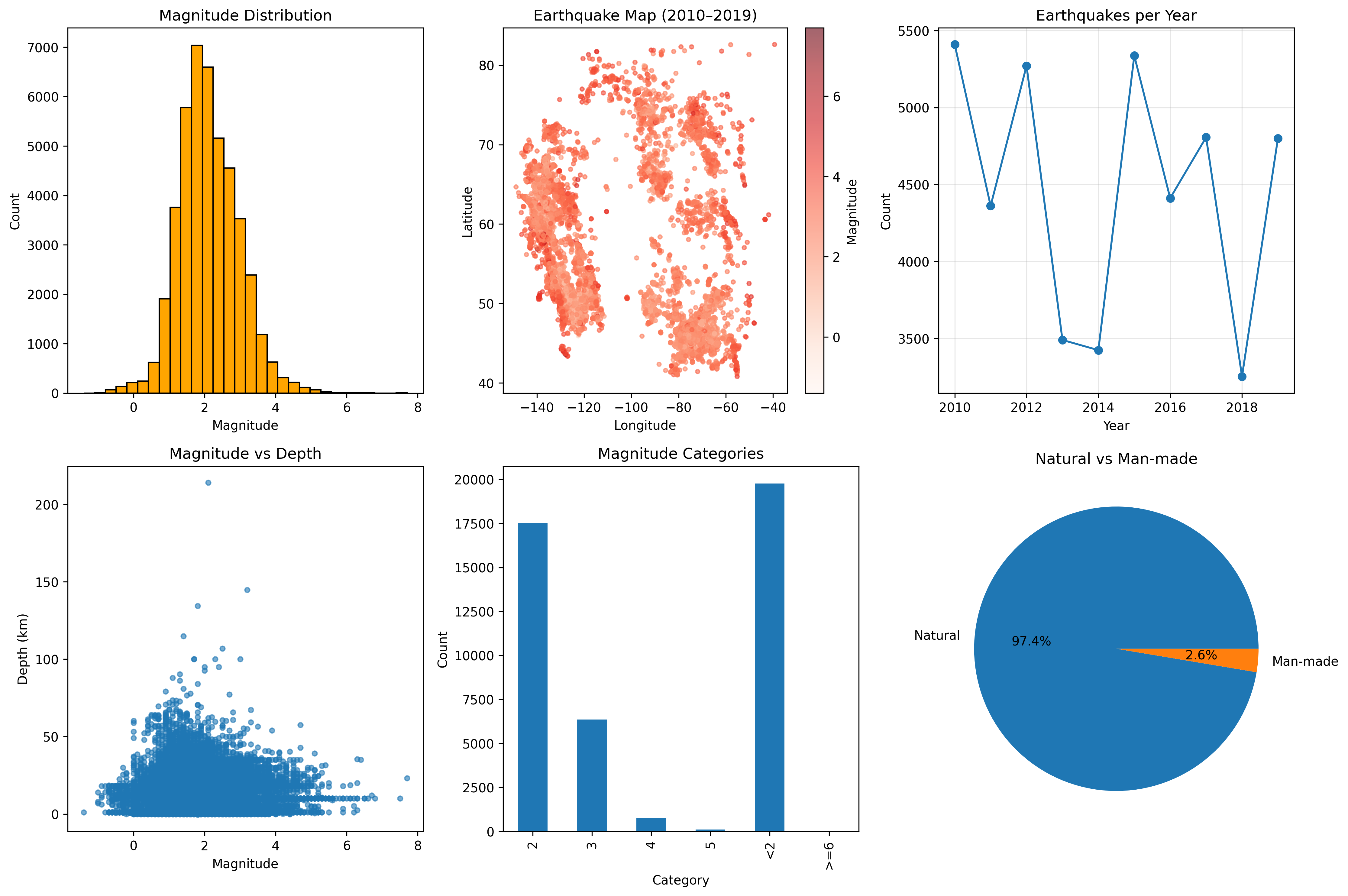
Refer to the following figure, choose two subfigures to reproduce with the earthquake dataset.

(In case you need this) Jupyter notebook setup

Visit https://docs.jupyter.org/en/latest/install/notebook-classic.html for some guidance to set up jupyter notebook.

Note: These notes are adapted from a blog post on Tom’s Blog.